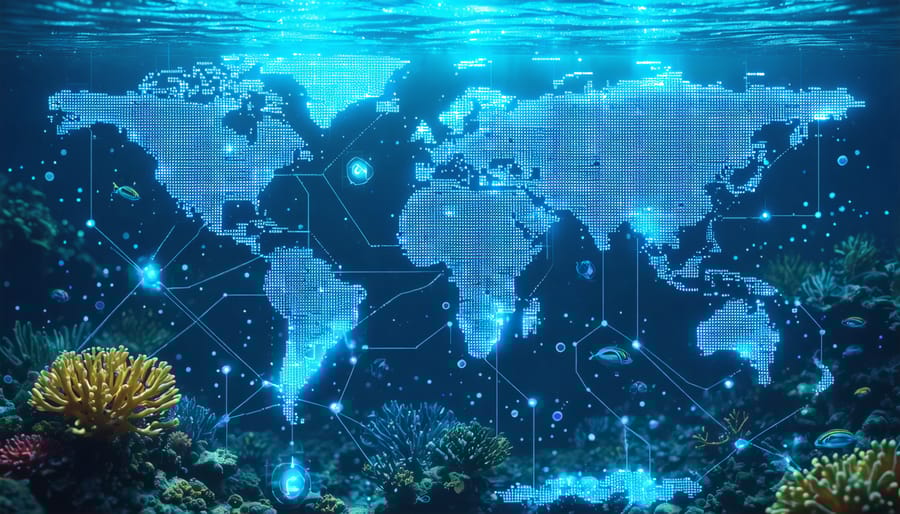
Harness the power of R’s spatial analysis capabilities to transform complex geographic data into actionable insights for marine ecosystem conservation and research. Modern environmental challenges demand sophisticated spatial analysis tools, and R provides an unparalleled open-source platform for processing, analyzing, and visualizing spatial data. Through packages like sf, sp, and raster, researchers can seamlessly integrate multiple data sources, from satellite imagery to species distribution models, creating a comprehensive understanding of marine spatial patterns.

The rise of big data in environmental science has made R’s spatial analysis capabilities increasingly crucial. Its ability to handle large-scale spatial datasets, perform complex geostatistical analyses, and create publication-quality visualizations has transformed how we approach marine spatial ecology. Whether mapping coral reef degradation, tracking marine mammal movements, or modeling climate change impacts on ocean ecosystems, R’s spatial analysis tools provide the flexibility and power needed for cutting-edge research.

This introduction to R spatial analysis will guide you through essential concepts, practical applications, and advanced techniques, enabling you to leverage R’s full potential for your environmental research. From basic spatial data handling to complex ecological modeling, you’ll discover how R’s ecosystem of spatial packages can enhance your research capabilities and contribute to more effective marine conservation strategies.

Essential R Tools for Marine Spatial Analysis

Core R Packages for Marine Analysis

R’s spatial analysis capabilities shine particularly bright in marine research through several specialized packages. The ‘sf’ (Simple Features) package serves as the foundation for handling vector-based spatial data, making it ideal for analyzing coastlines, marine protected areas, and vessel tracking data. Its modern approach to spatial data management integrates seamlessly with the tidyverse ecosystem, making species interaction analysis more intuitive and efficient.

The ‘sp’ package, while older, remains crucial for marine researchers working with legacy datasets or specific analytical tools. It excels in handling complex spatial data structures commonly found in oceanographic studies, such as depth profiles and current patterns.

For working with gridded data like sea surface temperature or chlorophyll concentrations, the ‘raster’ package is invaluable. It efficiently processes large satellite imagery datasets and enables sophisticated spatial analyses of marine environmental variables. The package’s memory-efficient operations make it possible to analyze vast ocean regions without overwhelming computational resources.

These core packages work together harmoniously, allowing researchers to combine different data types – from point observations of marine species to continuous environmental variables. When used alongside specialized marine science packages, they create a powerful toolkit for understanding ocean ecosystems and supporting evidence-based conservation decisions.

Data Visualization Techniques

R offers powerful tools for creating compelling spatial visualizations that help tell the story of marine ecosystems. The ggplot2 package, combined with specialized spatial packages, enables researchers to create informative maps and plots that illuminate patterns in marine data.

For basic spatial visualization, ggplot2’s geom_sf() function creates clear, publication-quality maps. You can enhance these maps by adding layers for different data elements, such as plotting coral reef locations as points or showing marine protected area boundaries as polygons. The scale_fill_viridis() function provides color palettes specifically designed for scientific visualization, making your maps both visually appealing and accessible.

To represent marine ecosystem patterns effectively, consider using:

– Heat maps to show species density or environmental variables
– Faceted maps to compare temporal changes
– Interactive plots using leaflet for web-based visualization
– Contour maps for showing depth or temperature gradients
– Bubble plots for representing species abundance

When visualizing marine spatial data, it’s essential to include proper map elements like scale bars, north arrows, and coordinate reference systems. The ggspatial package provides these cartographic elements, helping create professional-looking maps that effectively communicate your findings.

For complex analyses, combining multiple visualization techniques can provide deeper insights. For example, overlaying species distribution data on habitat maps can reveal important ecological relationships and support marine conservation planning efforts.

Case Studies: Tracking Marine Disturbances

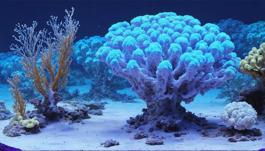
Coral Bleaching Events

Analyzing temporal patterns in coral bleaching events has become increasingly crucial as our oceans face unprecedented challenges. Using R’s spatial analysis capabilities, researchers can track and visualize the progression of bleaching events across reef systems over time, providing valuable insights into the health of these vital ecosystems.

Marine scientists commonly employ time series analysis in R to detect changes in coral reef conditions. By combining satellite imagery with in-situ temperature data, researchers can create detailed maps showing the spread and intensity of bleaching events. These visualizations help identify hotspots of coral stress and predict areas at risk of future bleaching incidents.

One powerful approach involves using R’s raster package to process remote sensing data, allowing scientists to track sea surface temperature anomalies – a key indicator of potential bleaching events. By analyzing these patterns over multiple years, researchers can identify recurring problem areas and seasonal trends that may contribute to coral stress.

The implementation of spatial autocorrelation techniques in R helps quantify the relationship between neighboring reef areas, revealing how bleaching events spread across connected reef systems. This information is vital for conservation planning and early warning systems.

Recent studies have demonstrated success in using machine learning algorithms within R to predict future bleaching events based on historical patterns. These predictive models incorporate various environmental parameters, including water temperature, light intensity, and ocean chemistry data, to forecast potential bleaching risks with increasing accuracy.

Citizen science initiatives have also benefited from R’s spatial analysis capabilities. Marine conservationists can now easily integrate volunteer-collected data with professional monitoring programs, creating more comprehensive datasets for tracking reef health over time. This collaborative approach has proven particularly valuable in regions where traditional monitoring resources are limited.

Through careful analysis of temporal patterns, scientists can better understand the factors driving coral bleaching and develop more effective conservation strategies to protect these endangered ecosystems for future generations.

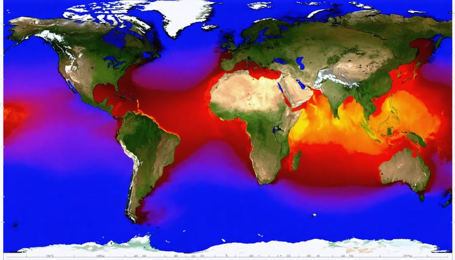
Ocean Temperature Anomalies

Ocean temperature anomalies represent crucial indicators of climate change impacts on marine ecosystems. Using R’s spatial analysis capabilities, researchers can effectively map and analyze these temperature variations across different oceanic regions and timeframes. The ‘raster’ package, combined with specialized oceanographic datasets, enables scientists to create detailed visualizations of sea surface temperature (SST) deviations from historical averages.

By implementing functions like raster::stack() and raster::calc(), analysts can process multiple temporal layers of temperature data, revealing patterns of warming or cooling trends. These analyses are particularly valuable when studying phenomena like marine heatwaves, which significantly impact coral reefs and fish populations. The integration of satellite-derived SST data with R’s spatial tools allows researchers to identify hotspots of unusual warming and track their evolution over time.

Understanding marine weather patterns and temperature anomalies helps scientists predict potential impacts on marine biodiversity. R’s ggplot2 package, combined with spatial functions, creates compelling visualizations that communicate these changes to both scientific and public audiences. Marine conservationists use these insights to develop targeted protection strategies for vulnerable areas.

Recent innovations in R packages have simplified the process of accessing and analyzing oceanographic data. The ‘rerddap’ package, for instance, provides direct access to NOAA’s ERDDAP servers, allowing researchers to download and analyze near real-time temperature anomaly data. This immediate access to current conditions enables rapid response to emerging marine conservation challenges and helps inform policy decisions aimed at protecting ocean ecosystems.

Marine Pollution Hotspots

Spatial analysis in R has become an invaluable tool for identifying and monitoring marine pollution hotspots across our oceans. By analyzing satellite imagery, water quality data, and vessel tracking information, researchers can create detailed maps that reveal patterns of pollution concentration and spread.

Using packages like ‘sf’ and ‘raster’, scientists can overlay multiple data layers to pinpoint areas where pollutants accumulate. These analyses often reveal surprising patterns, such as how ocean currents concentrate plastic debris in certain regions or how industrial discharge creates zones of elevated chemical contamination.

One powerful application is the tracking of oil spills and chemical releases. By combining real-time monitoring data with oceanographic models, researchers can predict the movement of pollutants and assess their potential impact on marine ecosystems. This helps emergency response teams act quickly and efficiently to contain environmental damage.

Citizen science initiatives have also embraced spatial analysis tools. Marine conservation groups use R to process data collected by volunteers who monitor beach pollution and water quality. This collaborative approach has led to the discovery of previously unknown pollution sources and helped authorities take targeted action.

The visualization capabilities in R are particularly useful for communicating findings to policymakers and the public. Heat maps and interactive plots clearly show how pollution levels vary across different areas and time periods, making complex data accessible to non-technical audiences.

Through continuous monitoring and analysis, these tools help identify trends and patterns that might otherwise go unnoticed, enabling more effective conservation strategies and pollution prevention measures.

Practical Implementation Guide

Data Preparation and Cleaning

Before diving into spatial analysis in R, it’s crucial to ensure your marine data is properly prepared and cleaned. Start by importing your spatial data using appropriate R packages like sf, sp, or raster, depending on your data format. Common marine spatial data formats include shapefiles for coastlines, CSV files with coordinates for species observations, and raster files for environmental variables.

When working with coordinate data, verify that all coordinates are in the same coordinate reference system (CRS). Marine datasets often use different projections, so you may need to transform them using st_transform() from the sf package. For global marine analyses, consider using equal-area projections like Mollweide or Lambert Azimuthal Equal Area to maintain accurate area measurements.

Check for and handle missing values in your dataset, which are common in marine surveys due to equipment malfunctions or challenging weather conditions. Use functions like is.na() to identify gaps, and decide whether to remove or interpolate missing values based on your research requirements.

Data validation is essential – look for impossible coordinates (like marine species recorded on land), outliers in measurements, and duplicate records. Create validation rules specific to your marine species or variables. For example, depth measurements should align with known bathymetric ranges for your study area.

Clean your attribute data by standardizing species names, removing special characters, and ensuring consistent units of measurement. When working with time series data, confirm that temporal resolution is uniform across your dataset.

Remember to document all cleaning steps in your R script with clear comments, allowing others to understand and reproduce your workflow. Creating a separate cleaning script helps maintain reproducibility and makes it easier to update when new data becomes available.

Analysis Workflow

The spatial analysis workflow in R typically follows a structured approach that begins with data preparation and ends with visualization of results. Start by importing your spatial data using packages like sf or sp, ensuring proper coordinate reference systems (CRS) are defined. Marine researchers often work with multiple data layers, including bathymetry, temperature, and species occurrence data.

Data cleaning comes next, where you’ll check for and handle missing values, outliers, and spatial inconsistencies. This step is crucial for maintaining data integrity, especially when dealing with complex marine datasets collected through various ecosystem monitoring techniques.

The analysis phase involves applying spatial statistics and modeling techniques. Common operations include:
– Creating buffer zones around marine protected areas
– Calculating distance matrices between sampling points
– Performing spatial interpolation for continuous variables
– Conducting hot spot analysis for species distributions
– Generating density maps of marine life observations

Visualization is integral throughout the process. Use ggplot2 with sf to create professional maps and spatial plots. Consider adding interactive elements with leaflet or mapview for dynamic exploration of your results.

Finally, document your workflow using R Markdown or Quarto, making it reproducible for other researchers. Include detailed comments about data sources, processing steps, and analytical decisions. This documentation helps maintain transparency and enables collaboration within the marine research community.

Remember to validate your results against field observations and consider the temporal aspects of your spatial data, as marine environments are dynamic systems that change over time.

Result Interpretation

When interpreting spatial analysis results, it’s crucial to consider both statistical significance and ecological relevance. Start by examining your spatial autocorrelation values, such as Moran’s I or Geary’s C, to understand the degree of clustering or dispersion in your marine data. Values closer to 1 indicate strong positive spatial correlation, while values near -1 suggest negative correlation.

For habitat distribution models, evaluate the model’s performance using metrics like AUC (Area Under the Curve) and TSS (True Skill Statistic). An AUC value above 0.8 typically indicates good model performance in predicting species distributions. However, remember that statistical significance doesn’t always translate to biological significance.

When analyzing marine protected area effectiveness, look for clear patterns in before-after comparisons and consider the spatial scale of your analysis. Changes in species abundance or diversity should be interpreted within the context of seasonal variations and natural population fluctuations.

Pay special attention to outliers in your spatial data – they might represent important ecological phenomena rather than errors. For example, unusual clustering of marine species could indicate essential habitat features or environmental stressors that warrant further investigation.

Finally, always validate your results against field observations and expert knowledge. Consider the temporal scale of your data and any potential sampling biases that might influence your conclusions. Remember that spatial patterns in marine ecosystems are often complex and may require multiple analytical approaches for robust interpretation.

R spatial analysis has emerged as an indispensable tool in advancing marine species conservation efforts, transforming how we understand and protect our ocean ecosystems. By enabling researchers to process vast amounts of spatial data and create detailed visualizations, R has revolutionized our ability to track marine species movements, monitor habitat changes, and identify critical areas for conservation.

The power of R spatial analysis lies in its versatility and accessibility. From mapping coral reef degradation to modeling the impacts of climate change on marine populations, these tools have provided invaluable insights that inform conservation strategies and policy decisions. The open-source nature of R ensures that researchers worldwide can collaborate, share methodologies, and build upon existing frameworks, fostering a global community dedicated to marine conservation.

Looking ahead, the future of R spatial analysis in marine conservation is exceptionally promising. Emerging technologies like satellite imagery, autonomous underwater vehicles, and environmental DNA sampling are generating unprecedented amounts of spatial data. R’s analytical capabilities will be crucial in processing this information and extracting meaningful patterns that can guide conservation actions.

The integration of machine learning algorithms with R spatial analysis tools is opening new frontiers in predictive modeling. This combination allows researchers to forecast marine species distributions, anticipate ecosystem changes, and develop proactive conservation measures. Additionally, the growing availability of user-friendly R packages makes these powerful analytical tools more accessible to conservation practitioners and citizen scientists.

As we face increasing challenges from climate change, ocean acidification, and habitat loss, R spatial analysis will continue to play a vital role in understanding and addressing these threats. By providing evidence-based insights and facilitating collaborative research, these tools empower conservationists to make informed decisions and implement effective protection strategies for our marine ecosystems.

The success of future marine conservation initiatives will depend heavily on our ability to harness and apply these analytical tools effectively. Through continued development and application of R spatial analysis, we can work together to ensure the preservation of marine biodiversity for generations to come.